The Motion of a Golf Ball

Usually, people, especially students, have issues with the concept that gravity is the only force acting upon an upward-moving projectile. Of course, gravity here refers to Newton’s theory). Their conception of motion prompts them to think that if an object moves in a given direction, there must be a force in that direction, e.g., if a particle moves upward and rightward, there must be both an upward and rightward force. Probably, they believe it is due to their intuition based on their daily lives, where the air resistance, often termed drag, might not be negligible. This tutorial shows the usage of the SimStack features to understand the importance of the air resistance effect on projectile motion.

Naturally, adding the drag force in the equations for a projectile motion is not complicated, but solving them analytically for position and velocity as functions of time can get tricky. Fortunately, it is relatively easy to make precise and accurate numerical solutions using Python’s Scipy library.

This project aims to show how the Projectile motion experienced by a Golf ball with mass $M (kg)$ and radius $r (m)$ projected near the Earth’s surface moves along a curved path under the action of gravity, $g=9.81 (m/s^2)$ when the effects of air-resistance and lift are assumed or neglected. Beyond the physics problems we aim to solve, we also want to highlight the loop control features of SimStack. With these features, we will submit several workflows with different setups for a given simulation protocol, which might be computed in parallel using the ForEach loop control and thus get the desired physical properties.

This tutorial demonstrates step-by-step through the Motion of a Golf ball project how to run and build simple and complex workflows. With these examples, we will learn how to iterate over parameter ranges using the ForEach loopcontrol. Additionally, we explain how workflows may be branched via If loop control.

Important

Please download all the WaNos for this project on Github.

In this workflow, we will be able to:

Understanding the connection of acceleration due to gravity, range, maximum height, and trajectory properties of a projectile motion.
Determine the velocity of a particle at different points in its trajectory.
Apply the principle of independence of motion to solve projectile motion problems when the effects of air resistance are assumed or neglected.

Theoretical Solution

The proper way to model the projectile motion is to split it into two independent motions, i.e., horizontal $(x)$ and vertical $(y)$. The magnitudes of the components of the velocity $V$ are $V_x = V cos(\theta)$ and $V_y = V sin(\theta)$ where $V$ is the magnitude of the velocity and $\theta$ is its angle direction, as depicted in Fig 1. Gravity, air resistance, and rotation (lift) affect a golf ball’s trajectory. We illustrate the forces acting on the ball on the right of Fig 2. This project will explore the following four scenarios: a smooth ball, smooth ball + drag, golf ball + drag, and golf ball + drag + lift.

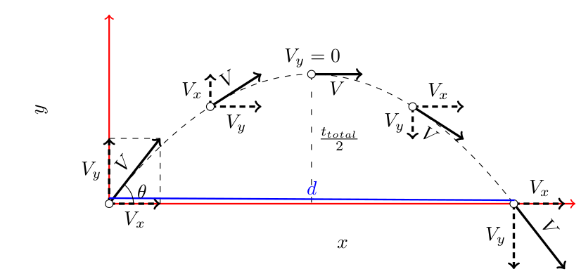
Fig 1 The split of a projectile motion into two independent one-dimensional motions along the vertical and horizontal axes. The horizontal range $d$ ( the blue line) is maximum distance traveled on the $x$ coordinate when it returns to its initial height ($y=0$).

2D General Equations

$F_x = - F^d_x + F^l_x$

$F_y = -F_g - F^d_x + F^l_y$

$F_g$ is the force of gravity that acts at all times on all objects near Earth.

The drag force or air resistance $F^d = \frac{1}{2}\rho_f A C_D|v|^2$ refers to forces acting opposite to the relative motion of the ball moving concerning a surrounding fluid (air in this case). Here, $C_D$ is the drag coefficient, ${\rho}$ is the air density, ${A}$ represents the cross-sectional area of the ball. The drag coefficient is not constant, it decreases as velocity increases.

$F^l = \frac{1}{2}\rho_f A C_L|v|^2$ is the lift force stemming from the rotation of the ball (the Magnus-effect) and is normal to $v$. With the given direction, the ball rotates counter-clockwise (backspin), where $C_L$ is the lift coefficient.

Projectile-motion WaNo

The Workflow building blocks within the SimStack Workflow framework are Workflow Active Nodes (WaNos), XML files combined with scripts defining the expected input and output. As pointed out above, we want to understand the physics of a Projectile motion with or without resistance effects; for that, we built a WaNo as shown in Fig 2, where only the relevant parameters are exposed.

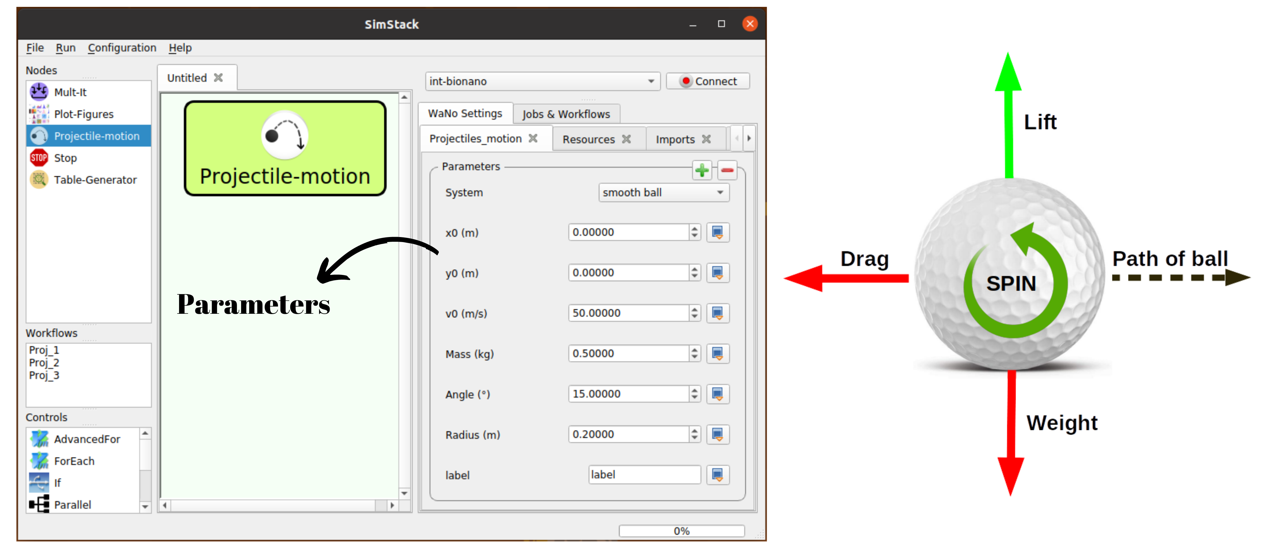
Fig 2 On the left-hand side is depicted the Projectile-motion WaNo . Outlined in blue we expose the most relevant physical parameters of the projectile motion problem. On the right-hand side, we depict some of the possible forces acting on the golf ball.

1. Python dependencies

To get this workflow up-running on your available computational resources, have the below libraries installed on Python 3.6 or newer.

Numpy, os, sys, csv, yaml
scipy
matplotlib

2. Inputs parameters with MultipleOf feature

Parameter	variable type
`System`	Boolean
`x0(m)`	Float
`y0(m)`	Float
`v0(m/s)`	Float
`Mass (kg)`	Float
`Angle(°)`	Float
`Radius(m)`	Float
`label`	String

The list above displays the Projectile-motion WaNo parameters with variable types and physical units. Here, $x_0$ and $y_0$ are the initial positions of the projectile in the horizontal and vertical axes. $v_0$ is the initial velocity. $Mass$ is the ball’s mass with a given Radius, and the label variable is a string to assign the chosen set of the variables. The System flag adds the desired scenario, and the equations of motion are solved numerically using the solve_ip from scipy library.

The set of the exposed parameters in this WaNo allows us to change the python script’s inputs without opening it. The outcomes follow the numerical solutions for the projectile motion within the chosen scenario.

3. Outputs

This WaNo will generate ` PROJOUT.yml` and `PROJDATA.yml` files. The table below shows the keys contained in each one, and later on, we will use these keys to inquire about their values.

PROJOUT.yml	PROJDATA.yml
xmax maximum range	$x$ position
ymax maximum height	$y$ position
time to target	$vx$ velocity
time to highest point	$vy$ velocity
Step ii label

4. Auxiliary WaNos

The Auxiliary WaNos set will be intensively used and reused in all upcoming workflows. They will be responsible for managing the outcome data. As shown in Fig 3, Mult-It, Plot-Figures, and Table-Generator will pass a variable at the beginning of the workflow and request the variable’s properties of a table file and plot figures.

Mult-It creates a Float or integer list, which will pass to the Projectile-motion WaNo inside the ForEach loop control, explained in the next step.
The Table-Generator WaNo generates table files in a csv and yml formats for a given set of variables inquired from a loaded file.
The Plot-Figures WaNo will make a plot of the inquired data. This WaNo allows us to switch between Same-graph (plot several curves in the same figure) and Subplot modes (plot each curve in a different subplot ).

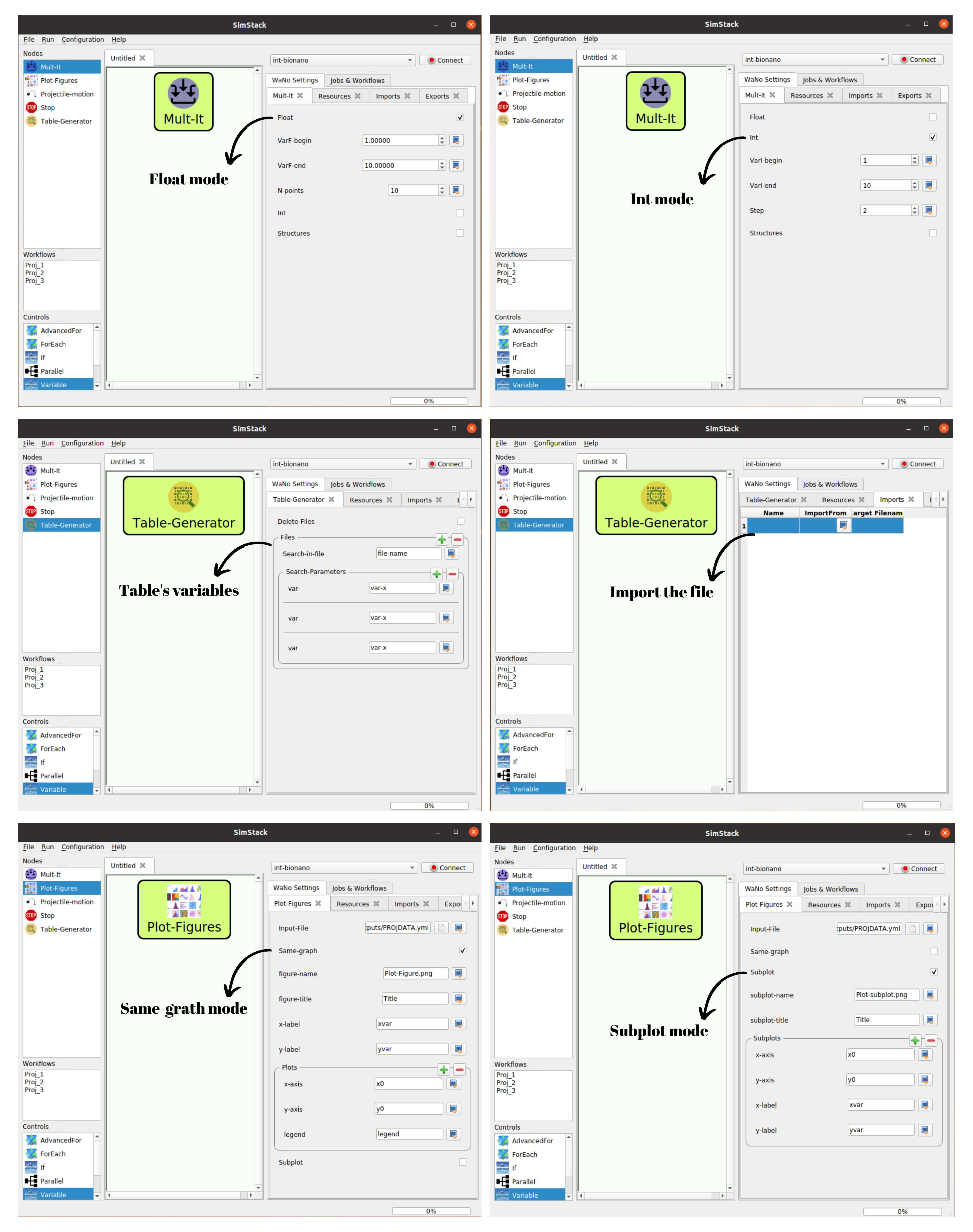
Fig 3 The upper two panels exhibit the Float and Int modes available on the Mult-It WaNo . The below two panels display the Same-graph and Subplot modes. Each mode in this WaNo allows us to inquire about the variables from Projectile-motion and plot them.

The outputs of the WaNo Plot-Figures in Fig 3 might be Plot-Figure.png and Plot-subplot.png . Click on Fig 3 to see more details about their inputs.

Workflow with Projectile-motion and Plot-Figures WaNos

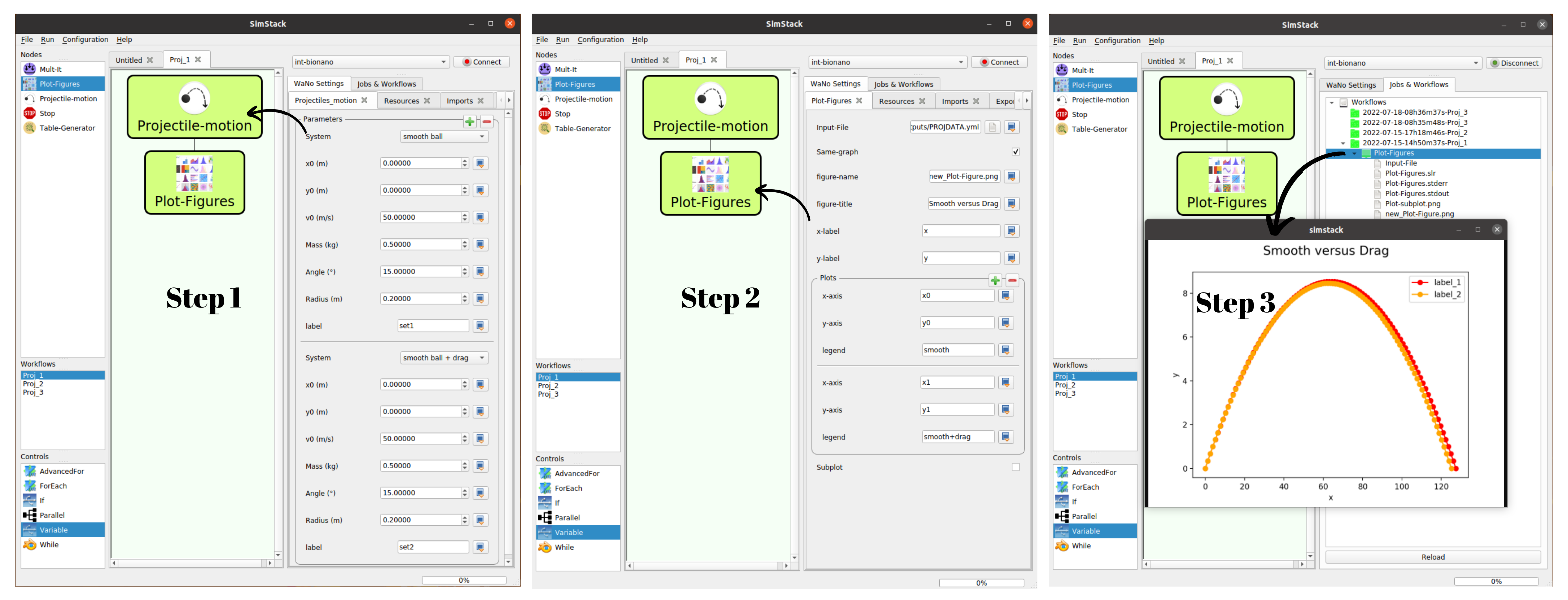
Fig 4 The workflow above is composed of Projectile-motion``*, and* ``Plot-Figures WaNos . Step 3 shows the figure as one of the possible outputs of this workflow.

Fig 4 shows the workflow named as Proj-motion, which compares the drag effect acting on a smooth ball.

5. Running this Workflow

Drag and drop the Proj-motion WaNo from the top left menu to the SimStack canvas as pointed by the blue arrow on panel Step 1 in Fig 4.
In this case, we set the Angle parameter to $25(°)$ for two different System scenarios (smooth ball and smooth ball + drag ), and we kept the other parameters as their default values.
Repeat Step 1 for auxiliary Plot-Figures WaNo connecting it below the Proj-motion. Load the PROJOUT.yml file field in the Input-File field, then click on the option Same-graph, the click will trigger the options to be filled. In this case, you should set the title, labels, and variables (data), which will show up in the output figure.
Name your workflow with Ctrl+S, and run it with Ctrl+R command.
The Step 3 of Fig 4 shows that by choosing the Browser Directory with a double click in the green folder (Jobs & Workflows tab) of the workflow, you will click on Plot-Figure.png and see the figure comparing the $x$ and $y$ coordinates of the smooth ball under or not of air resistance effect.

A slightly complex workflow using the ForEach feature

In this Workflow, we want to explore the scenario where the system under study has multiple initial velocities ($v_0$) values, and we want to investigate the dependence of maximum height $ymax$ and time to target variables in terms of maximum range $xmax$. For this example, the chosen system is golf ball + drag + lift.

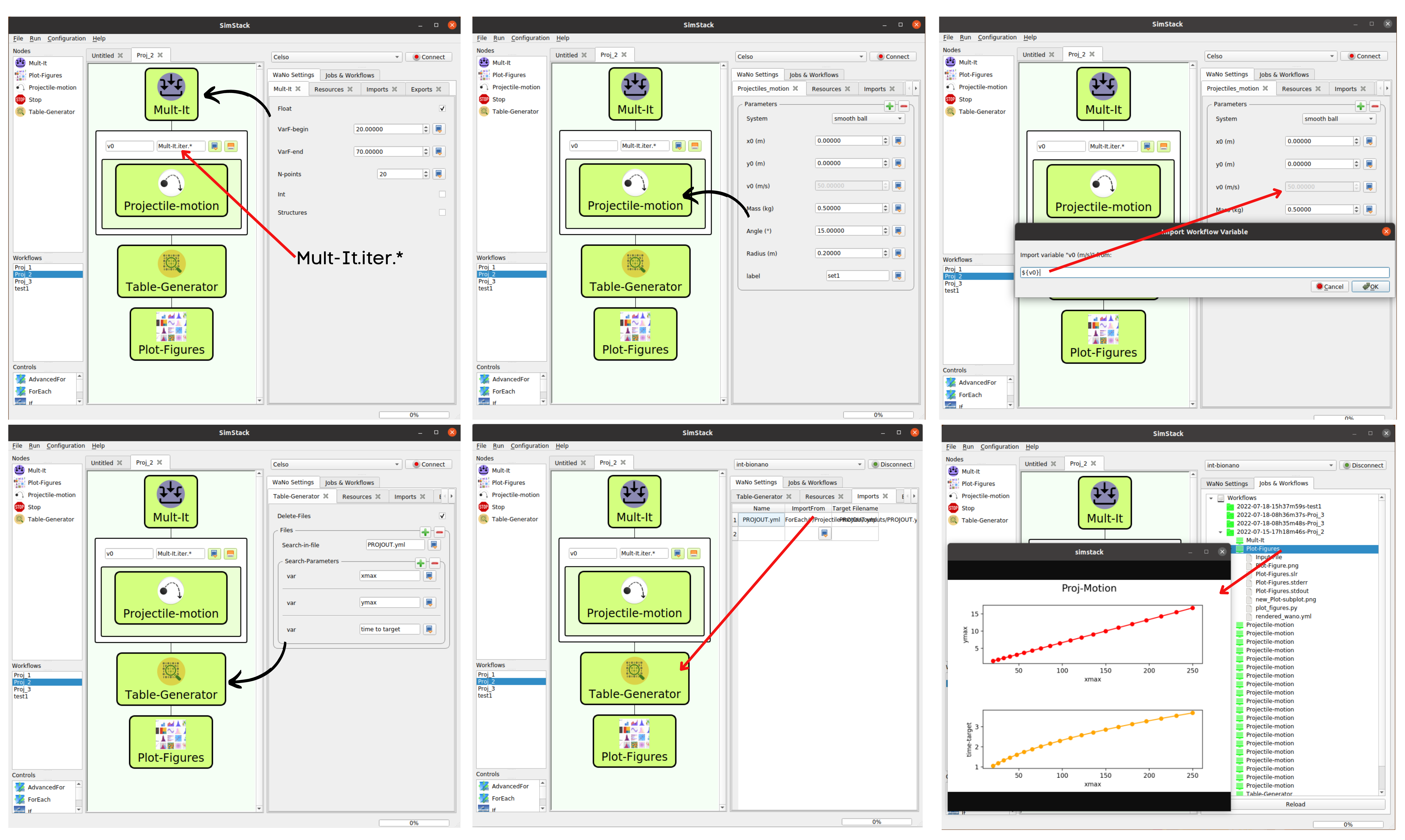
Fig 5 shows the workflow, a workflow composed of four WaNos and the ForEach loop control. The black arrows refer to the input parameters of each WaNo. The red arrow in Step 1 shows how to fill the field responsible for passing the list of values from Mult-It WaNo to the ForEach. The red arrow in Step 3 points out the assignment of the ForEach-Iterator to the initial velocity ($v_0`*) variable. The red arrow in* **Step 5** *shows the path to import all the files* ``PROJOUT.yml`$ of each initial velocity value. The last red arrow in Step 6 indicates the tab where we must browser to access the Plot-subplot.png figure.

6. Running this Workflow

Drag and drop the Mult-It WaNo from the top left menu to the SimStack canvas as pointed by the black arrow on panel Step 1 in Fig 5. There are 20 different values for initial velocity in this scenario, varying from 20 to 70 (m/s).
Drag and drop the ForEach loop control below right and insert the Projectile-motion WaNo inside it. In the sequence, assign the ${ForEach-Iterator} according to the Step 3 of Fig 5.
Drag and drop the Table-Generator WaNo from the top left menu to the SimStack below to ForEach loop control. Fill up the fields of Table-Generator as shown in Step 4 of Fig 5. You should also import the files from where the information will be extracted, in this case, PROJOUT.yml as depicted in Step 5.
Drag and drop the Plot-Figures WaNo from the top left menu to the SimStack below to Table-Generator, click on the option Subplot. In this case, you should set the title, labels, and variables (data), which will appear in the output figure. Fill the fields according to Step 6 of Fig 5.
Name your workflow with Ctrl+S, and run it with Ctrl+R command.
The last step in Fig 5 shows that by choosing the Browser Directory with a double click in the green folder (Jobs & Workflows tab) of the workflow, you will be able to click on Plot-subplot.png and see the subplots comparing the dependence of maximum height ymax and time to target variables in terms of maximum range xmax.

Branched Workflows using the If feature

This part will explain preventing unphysical results using the If loop control, which branches the workflow. In the Projectile-motion WaNo the options golf ball + drag and golf ball + drag + lift in the System field are only valid for initial velocities $v0(m/s)$ between $13.7$ and $88.1 m/s$. This constraint occurs due to the dependence of the drag and the lift coefficients, which are functions of the initial velocities and the golf ball spinning. In this case, we are keeping the spin constant. Then only the velocity will be considered.

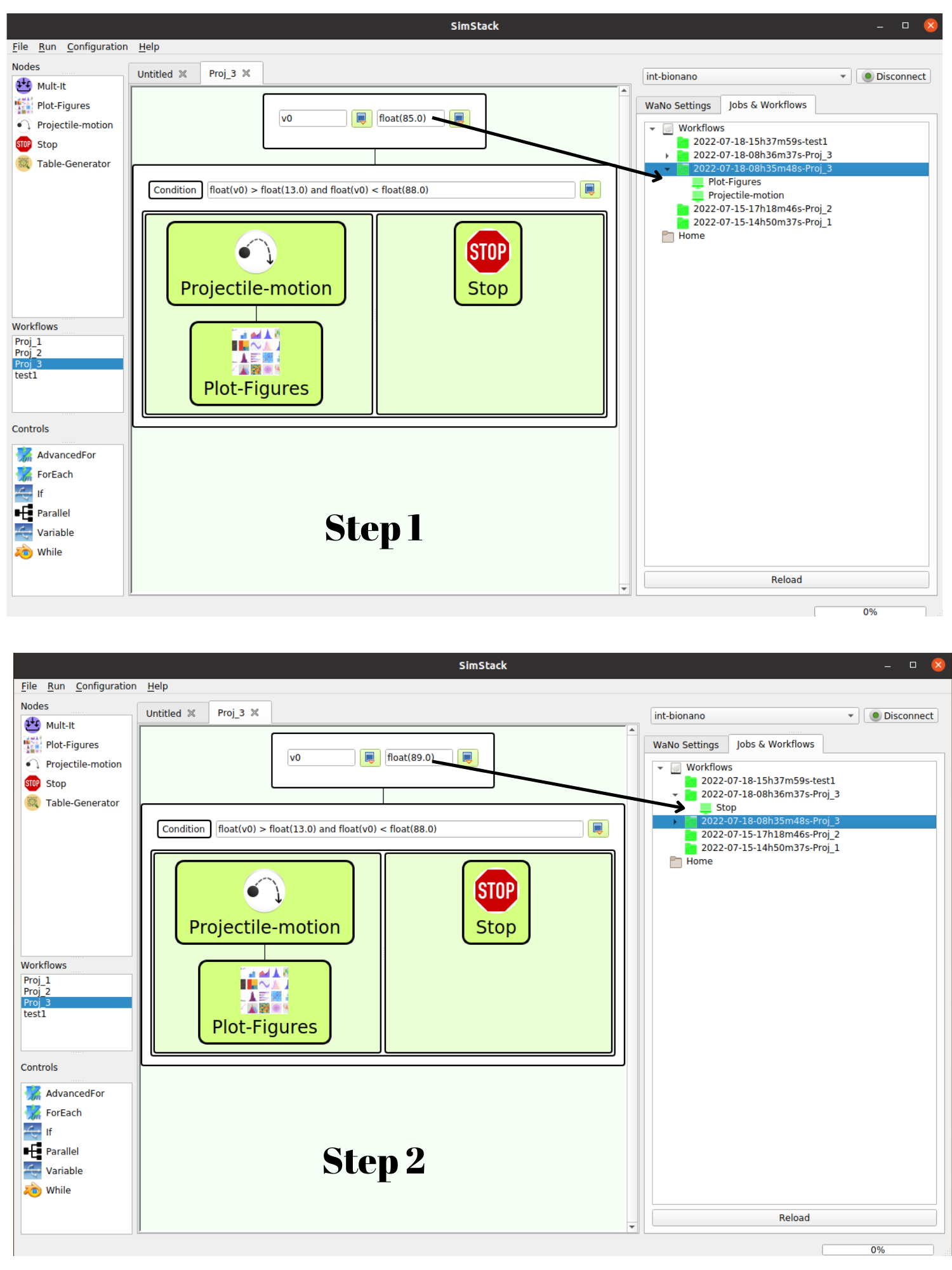
Fig 6 shows a branched workflow, which prevents unphysical results for a specific variable. The black arrows in both steps point from the variable $val_v0$ value to two different scenarios inside the If loop control.

Fig 6 exhibits the outcomes from this example. The workflow left and right sides display two possible scenarios for this case. (1) runs the workflow composed of the Projectile-motion and Plot-Figures or runs Stop WaNo, which prints a message on the Stop-msg file.

7. Running this Workflow

Drag and drop the Variable control from the bottom left menu to the SimStack canvas and setup it as shows Fig 6.
Drag and drop the If control bottom left menu and insert on the left-hand side the workflow composed by the Projectila-motion and Plot-Figures WaNos. Next, we make the appropriate setup for them. If this part is true, it must generate the expected output files for each WaNo as explained in section 5.
Drag and drop the auxiliary Stop WaNo from the bottom left menu inside the right side of the If loop control. If this part is true, it must generate the Stop-msg file.
Name your workflow with Ctrl+S, and running it with Ctrl+R command.
A double click in the green folder (Jobs & Workflows tab) of the workflow will allow us to check the outputs according to the chosen if condition.

Final Remarks

Running this project within SimStack saves time and avoids adding more code lines to our python script. For instance, to get the figure in Step 6, we would have to add a for loop in the python script to be executed in a serial version unless you want to make an additional effort to parallelize this task. On the other hand, SimStack promptly parallelize the jobs by running them onto the available computational resources. If we can leverage this advantage in a simple case, imagine how much time you can save for a more complex workflow involving different codes designed to simulate systems on different scales.