DFT convergence tests
In density functional theory (DFT) calculations, convergence tests of ENCUT and KPOINTS are crucial for obtaining accurate results. However, these tests are often neglected during the modeling phase since they require the submission of many short-time jobs, which require extensive expertise in scripting and command-line execution to handle the I/O files, which might be an issue for new users. We address this drawback by using workflow tools to manage the DFT calculations, which automate the process of performing convergence tests and ensure that the calculations are performed correctly. This can help to improve the accuracy and reliability of DFT results and prevent errors or inaccuracies in published research.
Here we use SimStack’s capabilities to calculate the properties of graphite with van der Waals corrections applied to the AB stacking structure. By employing the WaNos: Graphire, Mult-It, DFT-VASP, QE-DFT, and DB-Generator tools, we can effortlessly set up the graphite lattice parameters and select the perfect DFT method using VASP or Quantum Espresso code.
The raw data from the DFT calculation is automatically parsed and stored in a human-readable, lightweight database in .yml format, which can be accessed from GitHub Repos using Google Colab. With the help of libraries like matplotlib, seaborn, and others, users can quickly search and filter the data based on specific criteria, allowing them to identify trends and patterns in complex systems. Overall, the SimStack framework makes it easy for users to gain valuable insights into the properties of graphite.
Important
Please download all the WaNos for this project on Github
In this workflow, we will be able to:
Determine the optimal cutoff energy and k-mesh in the Brillouin zone.
Check the role and impact of the vdW correction when combined with GGA functionals.
Compute the Graphite lattice parameters deviation compared with the experimental values.
Graphite Convergence Tests
The figures below show the Convergence Tests workflow for the Graphite system. It comprises four WaNos and the AdvancedFor loop control, where we can toggle the encut and kpoints parameters as we wish. The black arrows link the input parameters of each WaNo; with this setup.
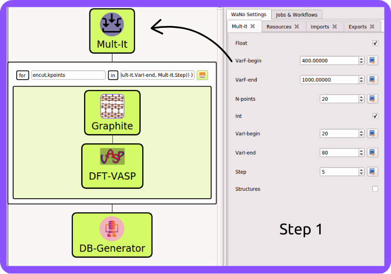
Fig 1 Step 1 is where the magic starts, and we are setting up the encut and kpoints list parameters. These lists will serve as input to the AdvancedFor loop control Mult-It.
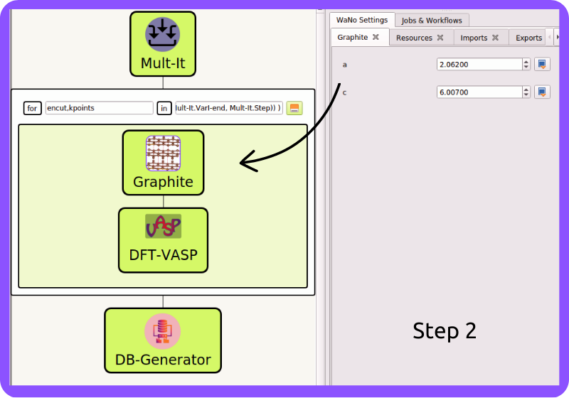
Fig 2 In Step 2, the Graphite lattice parameters are set to generate the POSCAR file Graphite.
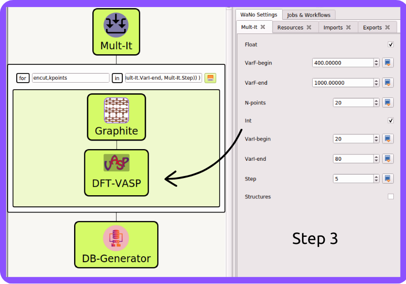
Fig 3 In Step 3, we set up the mandatory VASP code input files as detailed in its documentation DFT-VASP.
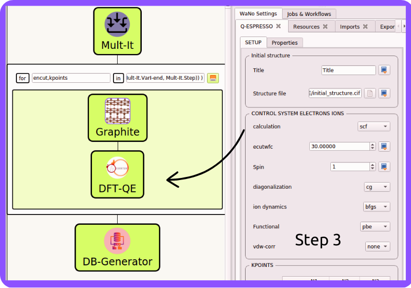
Fig 4 In Step 3, we set up the mandatory Quantum Espresso code input files as detailed in its documentation DFT-QE.
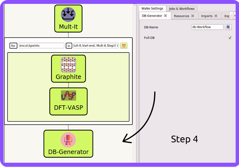
Fig 5 In step 4, we carefully craft a lightweight and easy-to-read database in .yml format for the entire workflow or a custom one for a specific subset of the WaNos, making it much more convenient for everyone to access DB-Generator.
It’s worth noting that we have two Step 3 options. If you do not have a VASP license (which is required by the DFT-VASP WaNo), you can opt to use DFT-QE instead, which utilizes the Quantum Espresso code as its backend. This way, you can still run DFT calculations without any limitations. It will give you more flexibility in choosing which DFT WaNo you prefer to work with.
1. Python dependencies
To get this workflow up-running on your available computational resources, have the below libraries installed on Python 3.6 or newer.
Atomic Simulation Environment (
ASE).Python Materials Genomics (
Pymatgen).glob,os,sys,re,yaml.Numpy,matplotlib.
2. Running this Workflow
Drag and drop the Mult-It WaNo from the top left menu to the SimStack canvas as showed in Fig 1 and set the parameters.
Drag and drop the AdvancedFor loop control below right, insert the Graphite WaNo inside it, and set the lattice parameters.
In the sequence, assign the encut,kpoints according to Fig 2 .
Drag and drop the DFT WaNo (VASP or QE) from the top left menu to the SimStack inside the AdvancedFor loop control. Set the fields you want to change.
Drag and drop the DB-Generator WaNo from the top left menu below to AdvancedFor loop control, and name your database.
Save and name your workflow with Ctrl+S, and run it with Ctrl+R command.
3. Outputs
This workflow will generate dB-Workflow (you can rename as you wish) files, human-readable
and lightweight databases in .yml format that can be easily accessed from GitHub Repos using Google Colab. These databases
are packed with all the workflow inputs and key parameters extracted from OUTCAR (main VASP output file) or
file.out (main Quantum Espresso output file), and you can use these keys to inquire about their values.
Results Analysis (GitHub & Google colab)
After running the workflow, we can download the databases to our GitHub repo and then quickly load them to our Google Colab account, where we can access and analyze our database to make the most out of our DFT simulations. We will explain how to do so below.
4. Cloning your GitHub repo
1import getpass
2username = getpass.getpass(prompt='GitHub username: ')
3password = getpass.getpass(prompt='GitHub password/Token: ')
4'!' git clone https://{username}:{password}@github.com/KIT-Workflows/Graphite-Workflow
5. Update your GitHub repo
1%cd /content/Graphite-Workflow
2'!'git pull
6. Querying properties of the database
 1import os, yaml
 2import numpy as np
 3import pandas as pd
 4import matplotlib.pyplot as plt
 5%matplotlib inline
 6
 7def filter_dicts(common_string, db_dict):
 8result = []
 9for key, value in db_dict.items():
10      if common_string in key:
11         result.append(key)
12return result
13
14if __name__ == '__main__':
15
16with open('db-d3bj-vdw.yml') as file:
17   db_file_encut = yaml.full_load(file)
18
19#print(db_file_encut["2023-01-04-16h34m57s-DFT-VASP_vasp_results.yml"])
20
21# Experimental lattice parameters for Graphite in AB staking
22a_0 = 2.462
23c_0 = 6.707
24
25common_string = 'DFT-VASP'
26prop_1 = 'ENCUT'
27encut = []
28kpoints = []
29prop_2 = 'total_energy'
30tot_energy = []
31a_lat = []  #'cell_lengths_and_angles'[0]
32c_lat = []  #'cell_lengths_and_angles'[5]
33
34
35results_dict_name = filter_dicts(common_string, db_file_encut)
36
37data_array = np.empty((0, 0))
38
39for dic_name in results_dict_name:
40      tot_energy.append(db_file_encut[dic_name][prop_2])
41      encut.append(float(db_file_encut[dic_name]["TABS"]["INCAR"]["ENCUT"]))
42      kpoints.append(float(db_file_encut[dic_name]["TABS"]["KPOINTS"]["Rk_length"]))
43      a_lat.append(db_file_encut[dic_name]['cell_lengths_and_angles'][0])
44      c_lat.append(db_file_encut[dic_name]['cell_lengths_and_angles'][2])
45
46data_array = np.append(data_array, encut)
47data_array = np.column_stack((data_array, tot_energy))
48data_array = np.column_stack((data_array, kpoints))
49data_array = np.column_stack((data_array, a_lat))
50data_array = np.column_stack((data_array, c_lat))
51
52# count the number of times that a given value appear in the first column of the array
53dim_array = data_array.shape
54
55# ENCUT
56count_encut = np.sum(data_array[:, 2] == data_array[0, 2])
57data_array = data_array[data_array[:,2].argsort()]
58
59# encut array
60encut_energies = np.empty((0, 0))
61encut_energies = np.append(encut_energies, data_array[dim_array[0]-count_encut:dim_array[0], 0])
62encut_energies = np.column_stack((encut_energies, data_array[dim_array[0]-count_encut:dim_array[0], 1]))
63encut_energies = np.column_stack((encut_energies, data_array[dim_array[0]-count_encut:dim_array[0], 2]))
64encut_energies = np.column_stack((encut_energies, data_array[dim_array[0]-count_encut:dim_array[0], 3]))
65encut_energies = np.column_stack((encut_energies, data_array[dim_array[0]-count_encut:dim_array[0], 4]))
66encut_energies = encut_energies[encut_energies[:,0].argsort()]
67
68# KPOINTS
69count_kpt = np.sum(data_array[:, 0] == data_array[0, 0])
70data_array = data_array[data_array[:,0].argsort()]
71
72# kpoints array
73k_energies = np.empty((0, 0))
74k_energies = np.append(k_energies, data_array[dim_array[0]-count_kpt:dim_array[0], 0])
75k_energies = np.column_stack((k_energies, data_array[dim_array[0]-count_kpt:dim_array[0], 1]))
76k_energies = np.column_stack((k_energies, data_array[dim_array[0]-count_kpt:dim_array[0], 2]))
77k_energies = np.column_stack((k_energies, data_array[dim_array[0]-count_kpt:dim_array[0], 3]))
78k_energies = np.column_stack((k_energies, data_array[dim_array[0]-count_kpt:dim_array[0], 4]))
79k_energies = k_energies[k_energies[:,2].argsort()]
Line 16 requires you to enter the name of your database.
7. Plotting the selected properties
 1# create a figure with a large size
 2fig, ax = plt.subplots(4,1,figsize=(20, 24))
 3ax[0].plot(encut_energies[:,0], (100*(encut_energies[:,3]-a_0)/a_0),'-ro')
 4ax[0].set_xlabel('ENCUT (eV)',Fontsize=20)
 5ax[0].set_ylabel(r'$\Delta a_{0}$ (%)', Fontsize=24)
 6ax[0].tick_params(labelsize=18)
 7ax[1].plot(k_energies[:,2], (100*(k_energies[:,3]-a_0)/a_0),'-ro')
 8ax[1].set_xlabel('KPOINTS (length (R_k))',Fontsize=20)
 9ax[1].set_ylabel(r'$\Delta a_{0}$ (%)', Fontsize=24)
10ax[1].tick_params(labelsize=18)
11ax[2].plot(encut_energies[:,0], (100*(encut_energies[:,4]-c_0)/c_0),'-ro')
12ax[2].set_xlabel('ENCUT (eV)',Fontsize=20)
13ax[2].set_ylabel(r'$\Delta c_{0}$ (%)', Fontsize=24)
14ax[2].tick_params(labelsize=18)
15ax[3].plot(k_energies[:,2], (100*(k_energies[:,4]-c_0)/c_0),'-ro')
16ax[3].set_xlabel('KPOINTS (length (R_k))',Fontsize=20)
17ax[3].set_ylabel(r'$\Delta c_{0}$ (%)', Fontsize=24)
18ax[3].tick_params(labelsize=18)
19plt.show()

The Colab notebook is available on the GitHub repository.
Final Remarks
The SimStack framework makes it a breeze for users to unlock valuable insights into the properties of a given system (Graphite, in this tutorial). By running this project within SimStack, you’ll save time and effort, and by connecting SimStack’s output with notebooks on Google Colab, you’ll be able to analyze your results with ease and grace like never before. Below we list several advantages to running a Python notebook on Google Colab.
1. Access to free GPU and TPU resources: Google Colab provides free access to GPU and TPU resources, which can significantly speed up computationally intensive tasks such as deep learning and machine learning.
2. Easy collaboration: Google Colab allows easy sharing and collaboration on notebooks. You can share a notebook with others and work on it together in real time.
3. Integration with Google Drive: Google Colab allows you to save your notebooks to Google Drive, which makes it easy to access your notebooks from anywhere and on any device.
4. Importing data: Google Colab can import data from various sources, including Google Drive, GitHub, and Kaggle. Pre-installed packages and libraries: Google Colab comes with many popular Python libraries pre-installed, such as TensorFlow, PyTorch, and sci-kit-learn, which can save you time and effort.
Easy-to-use interface: Google Colab provides an easy-to-use interface, which makes it accessible to users of all skill levels.
6. No setup or installation required: Google Colab requires no configuration or installation, making it easy to start. All you need is a web browser and an internet connection.
Note
Congratulations on completing this tutorial! You’ve now taken the first step in unlocking the power of the SimStack framework and Google Colab.